FDTD Optics Lab — User Guide
FDTD Optics Lab is a browser-based simulator for wave optics. It solves Maxwell's equations directly with the finite-difference time-domain (FDTD) method, so diffraction, interference, refraction, reflection, focusing and guiding all appear by themselves from the physics rather than from ray rules or textbook formulas.
It is designed for teaching, quick exploration and simple device design: choose an experiment, watch light propagate, compare the measured far-field pattern with analytic theory, or send a broadband pulse through a thin-film stack, Bragg mirror, guided-mode-resonance filter or waveguide grating and Fourier-transform the result into a transmission and reflection spectrum. Everything runs locally in the browser; there is nothing to install and no data leaves your computer.
01Quick start
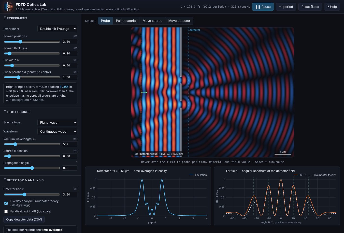
- Open the simulator. It starts running the Double slit (Young) experiment at λ₀ = 532 nm. Waves enter from the green dashed source line on the left.
- Wait a few periods. The clock in the top bar shows elapsed time in femtoseconds and optical periods. After roughly 40–60 periods the pattern is steady.
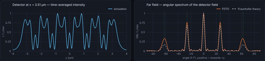
- Read the charts. The left chart is the intensity along the blue dotted detector line; the right chart is the far-field angular pattern with the dashed Fraunhofer theory on top.
- Change something. Drag the Slit separation d slider and watch the fringes tighten or spread. Parameter changes take effect immediately — the field keeps running.
- Try another experiment from the Experiment menu. Each one loads sensible source and detector settings plus an info box with the relevant theory.
02The interface
Top bar
| Element | What it does |
|---|---|
| Time readout | Simulated time in fs, number of optical periods elapsed, and simulation speed in time-steps per second. |
| Pause / Run | Stops or resumes time-stepping. Same as Space. |
| +1 period | Advances exactly one optical period (useful while paused). |
| Reset fields | Sets every field to zero and restarts the clock, keeping all settings. Use it to relaunch a pulse. |
| ? Help | Opens this guide in a new tab. |
Control panel sections
| Section | Contents |
|---|---|
| Experiment | Preset menu, its geometry parameters, and an info box with live theory (fringe angles, focal length, reflectance…). |
| Light source | Source type, CW or pulse, wavelength, position, angle, beam width and focus. |
| Spectrum (pulse + Fourier) | Wavelength range, monitor positions, frequency points, run length, stop criterion, axis and dB options. |
| Export results (CSV) | Save a plot-ready data file plus a matching specs file with every parameter and the device structure (details). |
| Detector & far field | Detector line position, Fraunhofer theory overlay, dB scale, copy data as CSV. |
| Grid & medium | Polarisation, y boundaries (absorbing or periodic), domain size, resolution (cells per λ₀), background index, PML thickness, grid statistics. |
| Display | Field vs. intensity view, brightness, auto-scaling, structure outlines, speed. |
| Draw materials | Brush material, index n and absorption κ, brush size and shape, undo and clear. |
| About the method | A compact technical summary (expanded in section 11). |
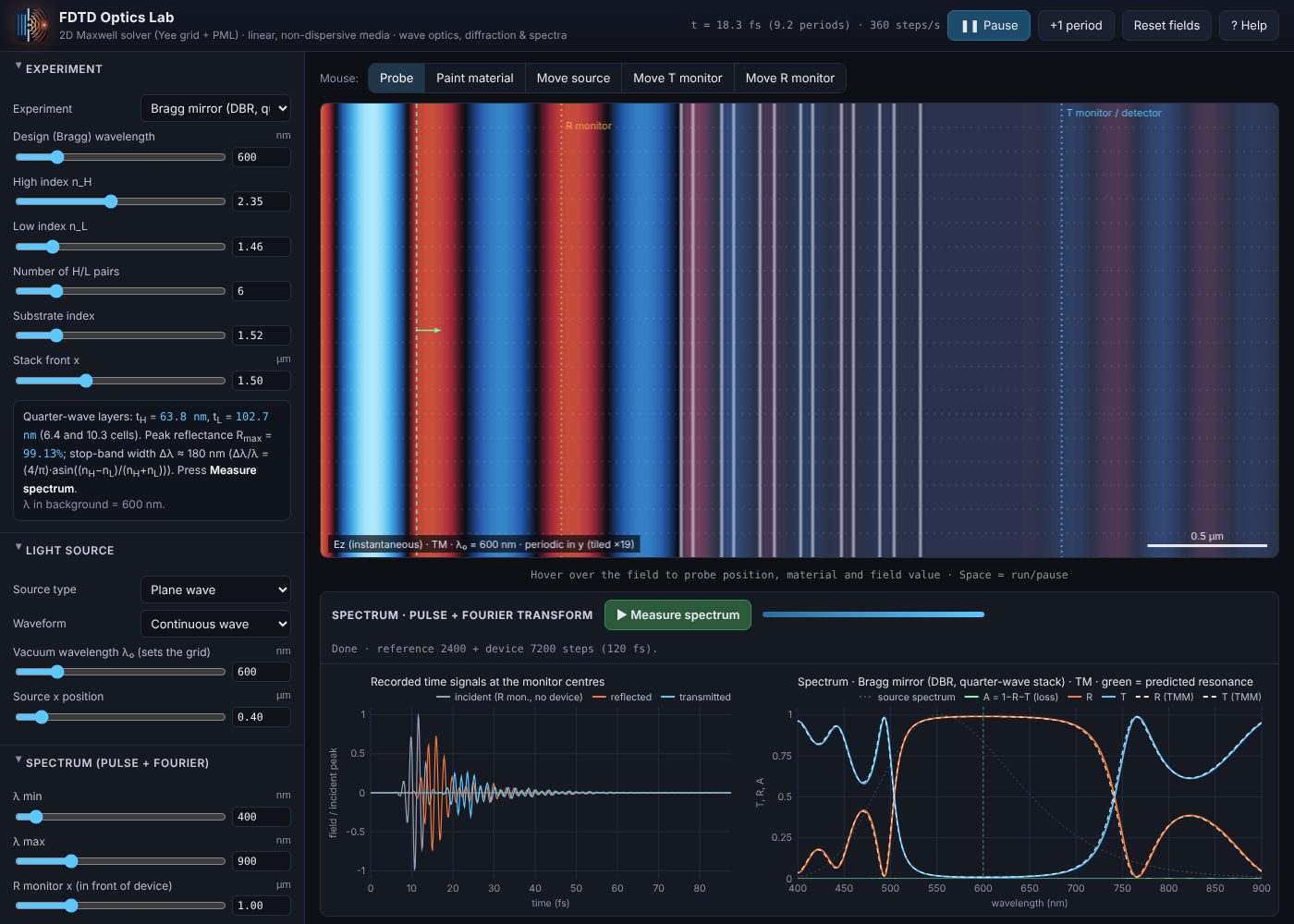
The spectrum panel below the field holds the ▶ Measure spectrum button, a progress bar and two charts: the recorded time signals and the spectrum.
Every slider has a number box next to it: type an exact value and press Enter. Typed values may exceed the slider's range where that makes physical sense.
Mouse tools
| Tool | Action on the field view |
|---|---|
| Probe | Hover to read position (µm), local material and the field value under the cursor. |
| Paint material | Click and drag to paint with the brush set in Draw materials. |
| Move source | Click to place the source. For a Gaussian beam the click also sets the beam centre; for a point source it sets x and y. |
| Move T monitor | Click to move the detector / transmission monitor line (blue) to that x position. |
| Move R monitor | Click to move the reflection monitor line (orange) used by spectrum measurements. |
On-screen markers: green dashed line = line source (with an arrow showing the propagation direction; a thick green bar marks a Gaussian beam's width), green circle = point source, blue dotted line = T monitor / detector, orange dotted line = R monitor. Material boundaries are outlined in white, dielectrics are lightly tinted and metals are solid grey.
03Experiments
Experiments are grouped into Diffraction & imaging, Refraction & guiding and Spectral devices. Choosing one resets the source, monitors, grid and spectral range to suitable values and restarts the fields. Your own drawings are kept (see section 7). All lengths are in micrometres; x runs left→right from the left edge of the visible domain, y is measured from the centre line (positive = up).
Single slit · Double slit · Diffraction grating
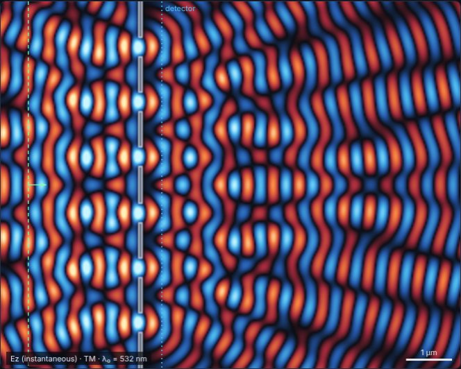
A perfectly conducting screen with one, two or N openings, illuminated by a plane wave. The far-field chart overlays the Fraunhofer prediction sinc² × array factor, and vertical green ticks mark the grating orders d(sin θm − sin θi) = mλ.
- Halve d and watch the orders move apart.
- Set d = 3a in the double slit: the 3rd order disappears (missing order).
- Tilt the plane wave with Propagation angle: the whole pattern shifts in sin θ.
- Make the slit narrower than λ/2 in TM, then switch to TE (see section 8).
Knife edge
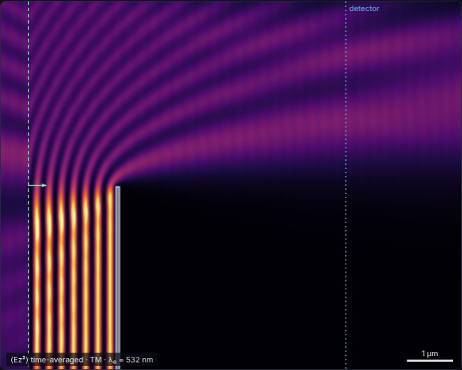
Half of the beam is blocked by a conducting half-plane. Behind it you see Fresnel edge diffraction: light leaks into the geometric shadow and fringes appear on the lit side, with a length scale √(λz/2) that grows with distance z.
- Move the detector further away and watch the fringes widen.
- Check that the intensity right at the shadow boundary is about ¼ of the unobstructed level.
Cylinder scattering
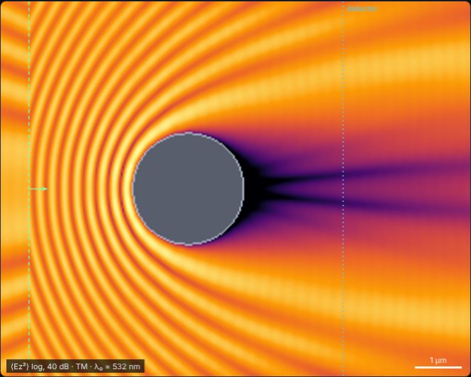
A dielectric or metal rod (seen end-on) in a plane wave. The info box gives the size parameter q = 2πr/λ: small rods scatter almost isotropically (Rayleigh), large rods cast a shadow with a strong forward diffraction lobe.
- Use Intensity, log scale to see the weak scattered field and the bright on-axis spot behind a metal cylinder (the 2D analogue of the Arago–Poisson spot).
- A dielectric rod with n ≈ 1.5–2 acts as a crude ball-lens and focuses light just behind it.
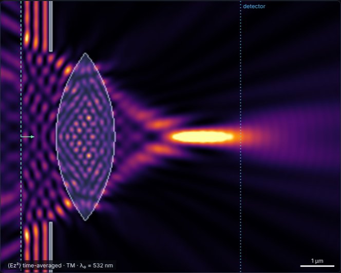
Cylindrical lens
A biconvex lens of aperture D, surface radius R and index n, optionally surrounded by an opaque stop. The info box reports the thick-lens focal length, back focal distance, NA and the expected diffraction-limited spot width; the detector is placed at the predicted focus.
- Compare the simulated focus with the paraxial prediction: strongly curved lenses focus short of it (spherical aberration).
- Reduce D: the focal spot becomes longer and wider (lower NA).
- Change n or the background index and watch the focus move.
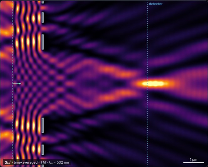
Fresnel zone plate
Alternate Fresnel zones are blocked so that all open zones add in phase at the design focus F. Zone radii are rm = √(mλF + (mλ/2)²).
- Look for the weaker higher-order foci at F/3 and F/5.
- Change the wavelength: a zone plate is strongly chromatic (F ∝ 1/λ).
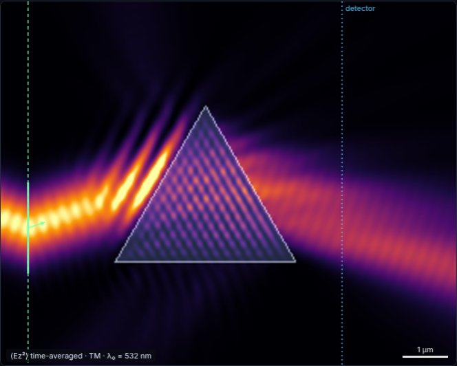
Prism
A triangular prism with apex angle α. The source beam is set automatically to the minimum-deviation incidence, and the info box reports δmin = 2θi − α. At minimum deviation the beam crosses the prism parallel to its base.
- Change the source angle by a few degrees either way: the deviation always increases.
- Raise n until the beam is totally internally reflected at the second face.
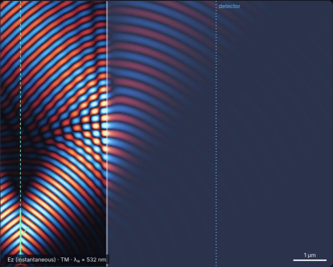
Interface: Snell, Fresnel, TIR, Brewster
A Gaussian beam hits a flat boundary between the background (nbg) and a second medium (n₂). The info box gives the refraction angle and the Fresnel reflectances Rs and Rp at the current angle, plus the Brewster and critical angles.
- Brewster: switch to TE (p-polarised), set the source angle to the Brewster angle — the reflected beam vanishes.
- TIR: set nbg = 1.5 and n₂ = 1.0, then exceed the critical angle (41.8°). The picture above shows TIR at 50° with the evanescent field just inside the second medium.
- Give medium 2 some absorption κ to model a lossy surface.
Slab waveguide
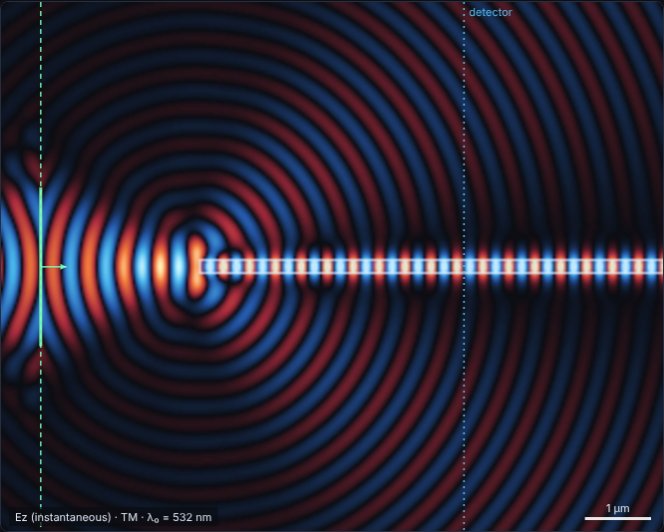
A high-index core guides light by total internal reflection. A focused Gaussian beam is launched into the entrance. The info box reports the numerical aperture, V-number and number of guided modes (single-mode when V < π/2).
- Widen the core: higher-order modes appear and the field inside shows a beating zig-zag pattern.
- Offset the core (Core offset y) to excite odd modes, or paint a bend with the brush and see how much light radiates away.
Free space / draw your own
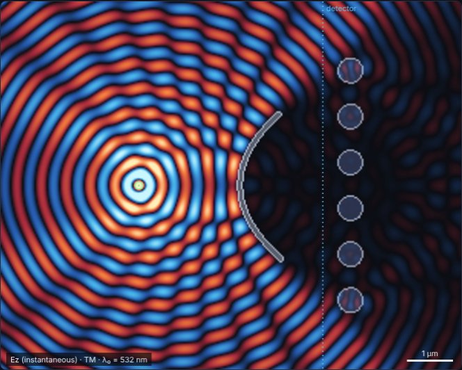
An empty domain with a point source. Use the Paint material tool to build any structure: mirrors, apertures, prisms, photonic crystals, gradient-index layers… Combine it with any source type. The picture shows a point source, a hand-painted curved metal mirror and a row of dielectric rods.
Thin film / Fabry–Pérot slab
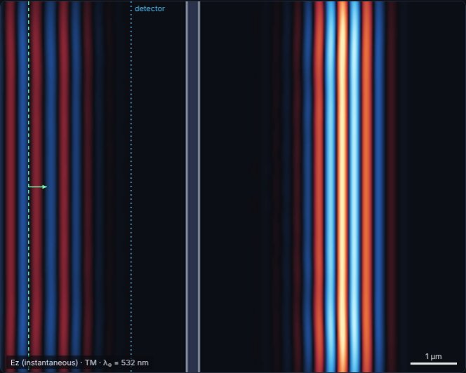
A dielectric layer of thickness t. With a continuous wave the standing-wave ripple in front of the slab shows the reflectance, which the info box calculates from the Airy formula. Quarter-wave thickness λ/4n maximises reflection; half-wave λ/2n makes the slab invisible.
- Switch the source to Gaussian pulse and press Reset fields: the pulse splits into a reflected and a transmitted part (shown above), and thick slabs produce a train of echoes.
- Set t = λ/2n and confirm the ripple disappears.
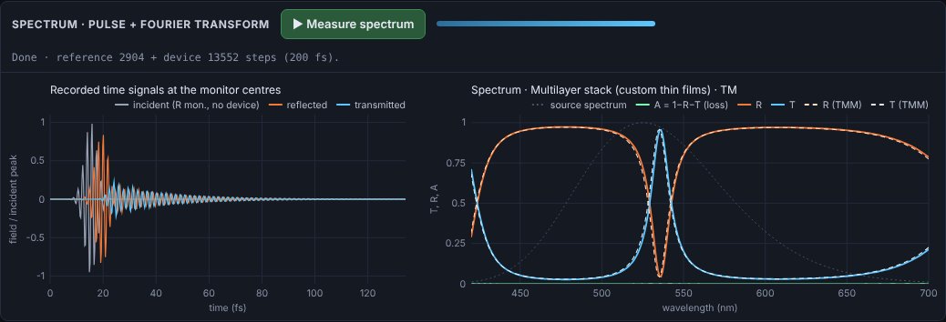
- Press Measure spectrum: R(λ) shows the Fabry–Pérot fringes, with the transfer-matrix result dashed on top.
Spectral devices
These presets are set up for spectrum measurement. Layered devices use periodic y boundaries, so the domain is only one period (or a thin slice) high and the picture is tiled vertically — they run in a second or two.
Multilayer stack (custom thin films)
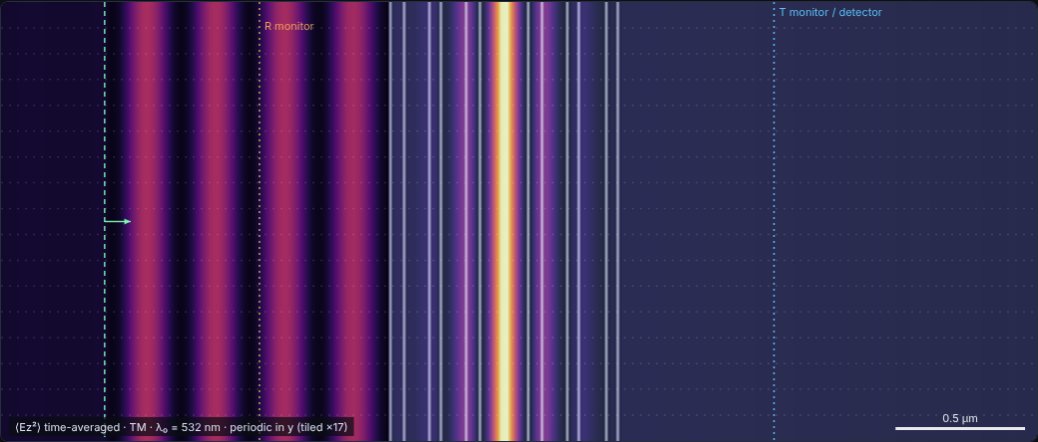
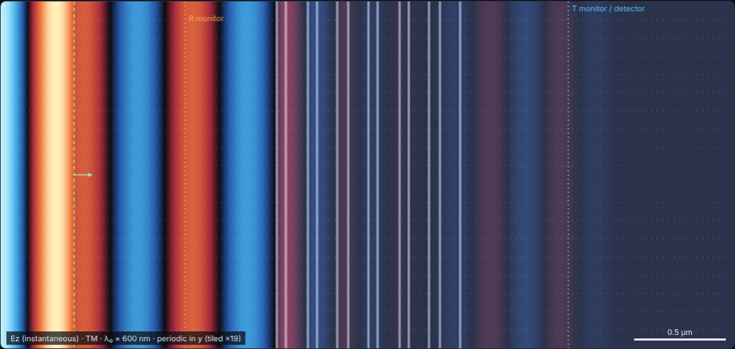
Type any stack of layers, incident side first, on a substrate of your choice. The default is a Fabry–Pérot bandpass filter: two TiO₂/SiO₂ quarter-wave mirrors around a half-wave spacer, transmitting a narrow band at 532 nm (the intensity builds up inside the spacer, as shown).
| Syntax | Meaning |
|---|---|
1.46:91.1 | layer of index 1.46, 91.1 nm thick |
2.0+0.05i:40 | absorbing layer, n = 2.0, κ = 0.05 |
(2.35:56.6 1.46:91.1)x5 | repeat the group 5 times (groups can be nested) |
Separate layers with spaces, commas or new lines; press Ctrl+Enter or click outside the box to apply. Try a single-layer anti-reflection coating: 1.38:96 on ns = 1.52.
Bragg mirror (DBR)
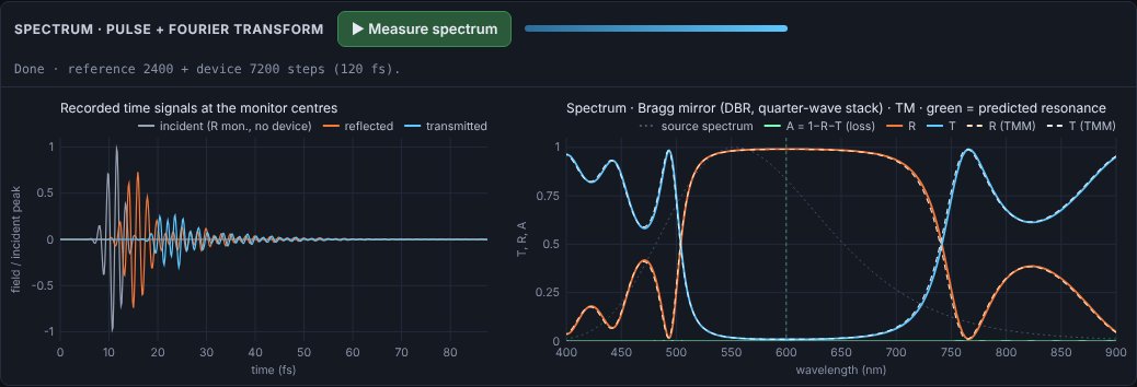
N pairs of quarter-wave layers (nH, nL) designed for λB. Reflections from every interface add in phase, giving a broad high-reflectance stop-band. The info box gives the layer thicknesses, the peak reflectance
and the stop-band width Δλ/λB ≈ (4/π)·asin((nH−nL)/(nH+nL)).
- Increase N: the stop-band gets flatter and closer to 100 %, its width stays the same.
- Reduce the index contrast: the stop-band narrows.
- Look for the third-order stop-band at λB/3.
Guided-mode resonance (GMR) filter
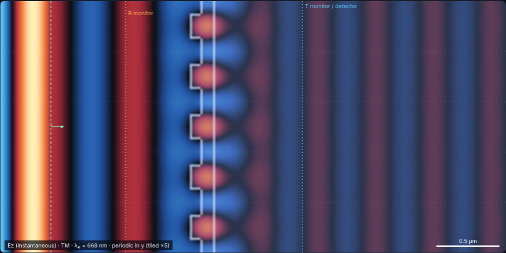
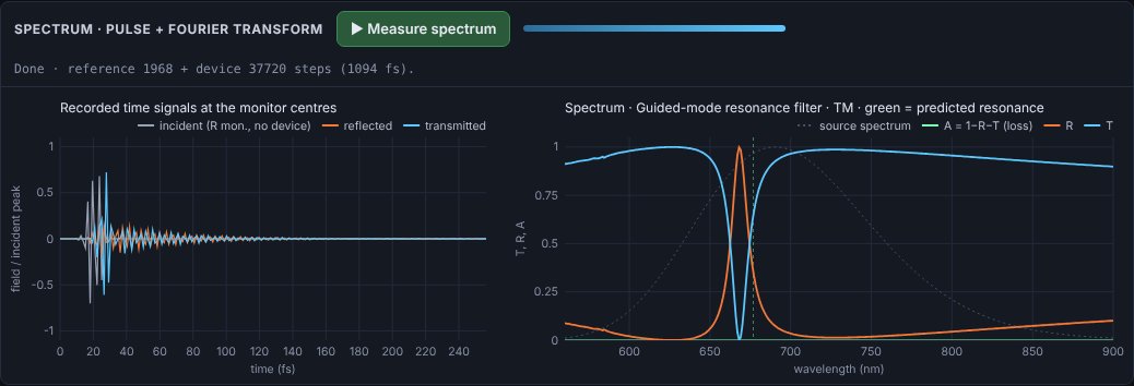
A sub-wavelength grating on a thin high-index waveguide layer. Normally incident light is diffracted into a guided mode when the period Λ satisfies Λ·neff(λ) = λ; the mode leaks back out and interferes with the directly reflected light, producing a narrow, nearly 100 % reflection peak. The image shows the strongly enhanced resonant mode trapped in the waveguide.
The info box estimates the resonance by solving the slab-waveguide mode equation (grating averaged into the film); the green line marks it on the spectrum. The default filter reflects > 99 % at 668 nm, about 1.3 % from that estimate.
- Reduce the grating thickness or fill-factor contrast: the resonance becomes narrower (higher Q) and needs a longer run.
- Change Λ: the peak tunes almost linearly.
- Switch to TE: a different mode (slab TM) gives a second resonance at another wavelength.
Waveguide Bragg grating
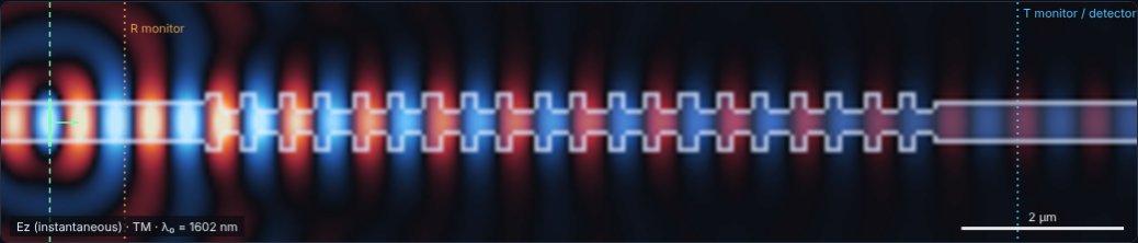
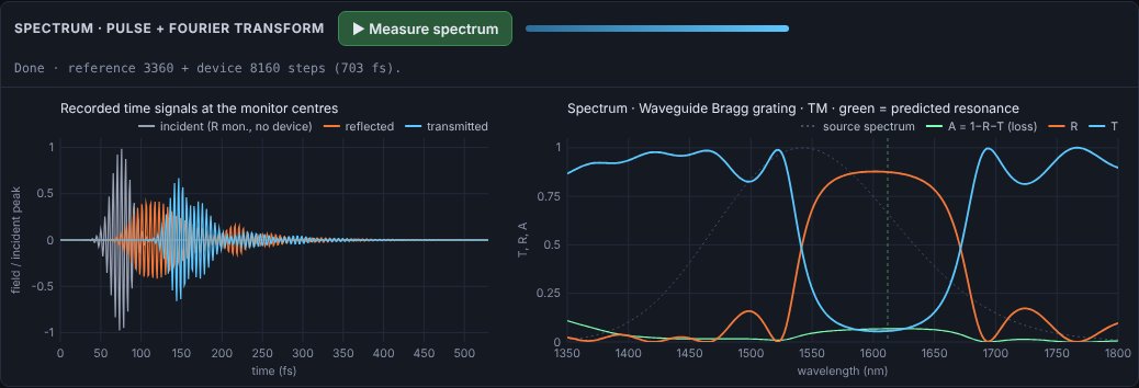
A silicon-nitride-like core in silica cladding whose width alternates every half period. The guided mode is reflected at the Bragg wavelength λB = 2·neff·Λ (neff from the slab mode solver, marked in green). The reference run uses a straight waveguide, so T and R are relative to the guided power.
- More periods: stronger, sharper reflection with side lobes.
- Smaller width modulation: weaker coupling, narrower stop-band.
- A = 1 − R − T here is light scattered out of the waveguide by the corrugation.
04Light sources
| Type | Description | Parameters |
|---|---|---|
| Plane wave | A vertical line source spanning the full height (into the absorbing boundaries), producing a uniform plane wave. | x position, propagation angle θ |
| Gaussian beam | A line source with Gaussian amplitude profile exp(−(y−yc)²/w²). A non-zero focus distance adds a converging phase so the beam focuses that far from the source line. | x, θ, radius w, centre yc, focus distance |
| Point source | A single-cell source radiating cylindrical waves (a line source along z in 3D). | x, y |
Waveform
- Continuous wave (CW) — a sinusoid at λ₀ switched on smoothly over three periods to avoid broadband transients. Use it for steady-state patterns and for the far-field analysis.
- Gaussian pulse — a carrier at λ₀ under a Gaussian envelope whose full width is set in optical cycles. Use it to follow wave-packets, separate multiple reflections or see transit delays. Short pulses are broadband; because materials here are non-dispersive, all frequencies see the same n. Press Reset fields to relaunch.
Angle convention
θ is measured from the +x axis; positive θ points towards +y (upwards). The angle is produced by a linear time delay along the source line, so it is exact for the plane-wave part of the beam. Angles above about 60° make the beam graze the top/bottom absorbers, which reduces quality.
05Spectra: pulse recording & Fourier transform
A single short pulse contains a whole band of wavelengths. Recording how it is reflected and transmitted, and Fourier-transforming the recordings, gives the full spectrum in one simulation — the standard way FDTD is used for device design.
Workflow
- Set the band in Spectrum (pulse + Fourier): λmin and λmax. The pulse is centred in this band and made just short enough to cover it.
- Place the monitors. The orange R monitor goes between the source and the device; the blue T monitor goes behind the device. Both must be in uniform material. Use the Move R/T monitor mouse tools or the sliders.
- Press ▶ Measure spectrum. Two runs follow automatically: a reference run without the device (records the incident pulse) and a device run. Each stops when the field at the monitors has decayed below the threshold (−80 dB by default) or at the maximum run length.
- Read the result. The left chart shows the recorded time signals; the right chart shows T, R, A and the source spectrum. Switch between wavelength and frequency, or linear and dB, at any time. Export with Copy CSV / Download CSV.
What is calculated
While the simulation runs, the electric and magnetic fields on every cell of both monitor lines are Fourier-transformed at all requested frequencies (a running DFT). The power flowing through each line is the Poynting flux:
Because powers (not field amplitudes) are compared, T and R are correct even when the transmitted light is in a substrate of different index, is diffracted into several orders, or travels in a waveguide. A is whatever is neither reflected nor transmitted through the T line: absorption in lossy materials, or light scattered sideways out of the domain.
Recorded time signals
The left chart shows the field at the centre of each monitor line, normalised to the incident peak: the incident pulse (R monitor, reference run), the reflected pulse (device run minus reference at the R monitor) and the transmitted pulse (T monitor). Long ringing after the pulse is the signature of a high-Q resonance; delays show group delay through the device. The time signals are included in the CSV export.
Settings
| Setting | Effect |
|---|---|
| λ min / λ max | Spectral band. A wider band means a shorter pulse. The grid must resolve λmin: the info box shows the cells per wavelength at λmin inside the densest material. |
| R / T monitor x | Monitor positions (µm). Keep the R monitor between source and device and the T monitor behind the device. |
| Frequency points | Number of wavelengths in the spectrum (uniform in frequency). More points cost proportionally more time during the run. |
| Max run length | Safety limit in optical periods of λ₀. If a run hits it before the field has decayed, the status line warns you and the spectrum may show ripples. |
| Stop when field decays to | −60/−80/−100 dB of the peak. Lower thresholds resolve sharper resonances. |
| Overlay TMM theory | For uniform layered structures (thin film, multilayer, DBR) the exact transfer-matrix result for the same, grid-rounded stack is drawn dashed. |
Exporting results (CSV)
The Export results (CSV) section — or the ⬇ Export CSV button in the spectrum panel — saves results as a pair of files sharing one name stem, e.g. fdtd_dbr_20261108-1400_spectrum.csv and fdtd_dbr_20261108-1400_specs.csv:
| File | Contents |
|---|---|
| …_spectrum.csv …_time.csv …_nearfield.csv …_farfield.csv | Plot-ready data: exactly one header row followed by numbers — no titles, comments or extra tables — so it loads in one line in any tool. Empty cells mean “no value” (e.g. T/R/A where the source spectrum is too weak). |
| …_specs.csv | Specifications: the data file names and the meaning and unit of every column; all experiment, device, material, grid, source, monitor and spectral parameters with units; derived design values (predicted resonance, layer thicknesses, peak reflectance…); the device layer table; the as-meshed index profile; and any drawn-material strokes. |
Data tables
| Data table | Columns |
|---|---|
| Spectrum | wavelength_nm, frequency_THz, transmittance, reflectance, absorptance, source_spectrum (+ transmittance_tmm, reflectance_tmm for layered devices) — sorted by increasing wavelength |
| Recorded time signals | time_fs, incident, reflected, transmitted |
| Detector near-field | y_um, intensity |
| Far-field pattern | theta_deg, far_field (+ fraunhofer_theory for slits and gratings) |
| All tables | One data file per table available (spectrum and time signals only after a measurement) plus one specs file. |
Copy data and Copy specs put either file on the clipboard; Preview shows the first lines of each file. In the browser you may be asked once to allow the site to download multiple files.
Plotting the data
# Python
import pandas as pd
df = pd.read_csv('fdtd_dbr_20261108-1400_spectrum.csv')
df.plot(x='wavelength_nm', y=['transmittance', 'reflectance', 'absorptance'])

% MATLAB
d = readtable('fdtd_dbr_20261108-1400_spectrum.csv');
plot(d.wavelength_nm, d.transmittance, d.wavelength_nm, d.reflectance)
Excel, LibreOffice and Origin open the data file directly with the column names in the first row.
06Detector & far-field analysis
The detector is a vertical line (blue, dotted) at position x. At every time-step it records two things for each cell along the line:
- Intensity ⟨F²⟩, where F is the out-of-plane field (Ez in TM, Hz in TE). For CW sources this is a running time-average over about three periods; for pulses it is the time-integrated energy. This is the left chart, normalised to its maximum.
- Complex amplitude U(y) at the source frequency, extracted by a running discrete Fourier transform (phase and amplitude).
The right chart is the angular spectrum of U(y), i.e. how strongly each plane-wave direction θ is present:
This is exactly the Fraunhofer (infinitely far) diffraction pattern of the field crossing the line. For slits and gratings under plane-wave illumination, the dashed curve shows the textbook result:
Why simulation and theory differ slightly
- The theory assumes an infinitely thin screen; the simulated screen has thickness, so each slit acts as a short waveguide. In TM this suppresses large angles; in TE it enhances them.
- The detector line has finite height, which slightly broadens peaks.
- Staircasing: slit widths are rounded to whole grid cells.
Exporting data
Copy detector data (CSV) puts both curves on the clipboard (y in µm with normalised intensity; θ in degrees with normalised far field and theory) for pasting into a spreadsheet, Python or MATLAB. The clipboard requires the page to be served over HTTPS or from localhost.
07Materials & drawing
Every grid cell holds a complex refractive index n + iκ at the source wavelength, or is a perfect electric conductor (PEC). The background index nbg (in Grid & medium) fills everything not otherwise specified.
| Material | Typical n (visible) | Notes |
|---|---|---|
| Air / vacuum | 1.00 | |
| Water | 1.33 | |
| Fused silica | 1.46 | |
| Crown glass / PMMA | 1.49–1.52 | |
| Flint glass | 1.6–1.8 | |
| Silicon nitride | 2.0 | use ≥ 20 cells/λ₀ |
| Titanium dioxide | 2.5–2.6 | use ≥ 30 cells/λ₀ |
| Silicon (at 1550 nm) | 3.48 | set λ₀ = 1550 nm, ≥ 40 cells/λ₀ |
| Metal | — | use Perfect conductor |
Absorption κ: a non-zero κ makes the material lossy; the intensity decays as exp(−4πκx/λ₀). κ must be smaller than n (it is clamped to 0.95 n). Real metals (κ > n, negative permittivity) are outside the model — use PEC instead.
Drawing
- Open Draw materials and choose the brush: Dielectric (with n, κ), Metal, or Eraser (resets to the background).
- Set the brush radius and shape (circle/square).
- Select Paint material above the canvas and drag. You can paint while the simulation runs.
- Undo stroke removes the last drag; Clear drawing removes all painting.
08Polarisation: TM and TE
The simulation is 2D: nothing varies along z. Maxwell's equations then split into two independent polarisations:
| Mode | Fields | Optics name | Shown on screen |
|---|---|---|---|
| TM | Ez, Hx, Hy | s-polarised (E ⟂ plane of incidence, parallel to slit edges) | Ez |
| TE | Hz, Ex, Ey | p-polarised (E in plane of incidence) | Hz |
Naming conventions for TE/TM differ between textbooks; this tool follows the common FDTD convention above. The physical consequences you can observe:
- Brewster angle (zero reflection) exists only for p-polarisation → TE.
- Narrow metal slits: in TM, Ez must vanish on the metal walls, so a slit narrower than λ/2 is below cut-off and transmits only evanescently. In TE, slits of any width transmit (a TEM-like mode).
- Fresnel reflectances differ: Rs ≥ Rp at every angle.
09Display
| View | Colour map | Best for |
|---|---|---|
| Instantaneous field | blue (−) · black (0) · orange (+) | Wavefronts, phase, wavelength in materials, propagation direction |
| Time-averaged intensity | black → purple → orange → yellow | Where energy goes: foci, fringes, shadows, standing waves |
| Intensity, log scale | same, over 40 dB | Weak scattered light, side lobes, evanescent tails, boundary quality |
- Auto-scale keeps the brightest ~0.5 % of the field just saturated. Turn it off to freeze the current scale, e.g. to compare two settings fairly.
- Brightness multiplies the scale by 2ⁿ; raise it to bring out weak features.
- Speed sets time-steps per animation frame. Higher is faster but less smooth.
10Grid, boundaries & accuracy
The grid spacing is Δx = λ₀ / Nλ, where Nλ is Cells per λ₀. Inside a material of index n the wavelength shrinks to λ₀/n, so the effective resolution there is Nλ/n.
| Cells per wavelength in the densest material | Quality |
|---|---|
| < 8 | Poor: large phase errors, waves visibly slower and direction-dependent |
| 10–15 | Good for qualitative demonstrations (default) |
| 20–30 | Quantitative: phase error ≲ 1 % over many wavelengths |
| ≥ 40 | High accuracy; slow for large domains |
A warning appears above the canvas when resolution inside the densest material falls below 10 cells per wavelength.
Cost
Run time scales with the number of cells, (W·H)/Δx², and the time to cross the domain scales with W/Δx — so doubling the resolution makes a run about 8× longer. The grid statistics in Grid & medium show the cell count. As a guide, ~100 k cells runs comfortably on a laptop; above ~700 k cells a warning appears.
Boundaries in y: absorbing or periodic
In x the domain is always closed by absorbing layers. In y you can choose (Grid & medium → y boundaries):
- Absorbing (PML) — an isolated structure in open space. Use for slits, lenses, scatterers and waveguides.
- Periodic — the domain height is one period of an infinite array; whatever leaves at the top re-enters at the bottom. Use for gratings, GMR filters and uniform layer stacks (which only need a thin slice). The field view is tiled vertically so you see several periods; faint dotted lines mark the period boundaries. Periodic mode supports normal incidence only — the source angle is ignored.
In periodic mode the domain height is divided into a whole number of cells, so the cell height Δy may differ slightly from Δx to represent the period exactly; the time-step adapts automatically.
Absorbing boundaries (PML)
The visible domain is surrounded by a perfectly matched layer, 20 cells thick by default, that absorbs outgoing waves with a design reflection of 10⁻⁶. Increase it to 30–40 cells if you see reflections in the log-intensity view (e.g. with grazing beams); decrease it for speed with small domains.
11The numerical method
Maxwell's equations in 2D (TM)
TE follows by exchanging the roles of E and H (duality).
Yee scheme
Fields are stored on a staggered grid: Ez at cell centres, Hx and Hy half a cell away in y and x, and E and H half a time-step apart (leapfrog). With normalised fields H̃ = η₀H and Courant number S = cΔt/Δx:
The scheme is stable for cΔt ≤ 1/√(1/Δx² + 1/Δy²) (S ≤ 1/√2 for square cells); the simulator uses cΔt = 0.5·min(Δx, Δy). With rectangular cells the factor S in the x- and y-difference terms becomes Sx = cΔt/Δx and Sy = cΔt/Δy. Perfect conductors are enforced by setting Ca = Cb = 0 for the tangential electric field.
Materials
In TE, permittivities for Ex and Ey are averaged over the two neighbouring cells to reduce staircasing errors at interfaces.
Perfectly matched layer
Berenger's split-field PML: the out-of-plane field is split into two parts (e.g. Ez = Ezx + Ezy), each damped only by the conductivity along its own direction. Electric and magnetic conductivities are matched (σ/ε = σ*/μ) so the layer is reflectionless at its interface for any angle and frequency in the continuum limit. The conductivity grows cubically with depth d:
Because matching uses the ratio σ/ε, structures that extend into the PML (screens, half-spaces, waveguides) remain absorbed correctly.
Spectral analysis
The source pulse is s(t) = exp(−((t − t₀)/τ)²)·sin(ωc(t − t₀)) with ωc at the band centre and τ = 3/Δω, so the source spectrum falls to about 10 % of its peak amplitude at the band edges. Every few time-steps (≥ 8 samples per period at λmin), each monitor cell updates
E and H are first interpolated to the same point in space and their half-step time offset is removed with a phase factor eiωΔt/2, so the flux ½Re∫Ẽ×H̃* is exact to second order. Frequencies whose reference power is below 0.1 % of the peak are left blank.
Transfer-matrix theory
For layered structures the dashed theory uses the characteristic-matrix method at normal incidence, applied to every grid cell between the monitors with complex index N(λ) consistent with the simulation's conductivity model:
Slab-waveguide mode solver
Resonance estimates for the GMR filter and waveguide Bragg grating come from the fundamental-mode dispersion equation of a three-layer slab (cover nc, film nf of thickness d, substrate ns), solved by bisection:
then λ is found from Λ·neff(λ) = λ (GMR, first order) or 2Λ·neff(λ) = λ (Bragg). This tool's TM polarisation (E along z, parallel to the layers) corresponds to the slab TE mode.
Units
| Quantity | Formula | Default value (λ₀ = 532 nm, Nλ = 16) |
|---|---|---|
| Grid spacing | Δx = λ₀/Nλ | 33.3 nm |
| Time-step | Δt = SΔx/c | 0.0555 fs |
| Steps per period | Nλ/S | 32 |
| Optical period | λ₀/c | 1.77 fs |
Because Maxwell's equations are scale-invariant, only ratios matter: a structure 10 µm wide at λ₀ = 1 µm behaves exactly like one 1 cm wide at λ₀ = 1 mm.
12Troubleshooting
- Nothing appears to come through my slit.
- In TM, slits narrower than half the wavelength (in the background medium) are below cut-off. Widen the slit or switch to TE. The info box warns about this.
- The far-field chart doesn't match the theory.
- Check that the source is a plane wave (theory assumes it), that the detector is just behind the screen in uniform medium, and that you have waited for a steady state. Small differences at large angles are expected (finite screen thickness, see section 6).
- The picture looks noisy or speckled at the start.
- That is the transient as the wave first fills the domain. Wait 30–60 periods, or press Reset fields after changing geometry drastically.
- Waves look jagged or travel at odd speeds inside a material.
- Resolution is too low for that index; raise Cells per λ₀ until the warning disappears.
- I see reflections from the edges.
- Increase the PML thickness, keep beams away from grazing angles, and move sources at least a few cells away from the boundary.
- The colours suddenly look dim.
- A very bright spot (e.g. near a point source or in a focus) sets the auto-scale. Raise Brightness or use the log view.
- It's slow.
- Reduce the domain size or the cells per λ₀, increase Speed (steps per frame), and close other heavy browser tabs. Chrome, Edge and Firefox all run it well; desktop is faster than mobile.
- The spectrum has ripples or wiggles.
- The run stopped before a resonance had finished ringing (the status line warns). Increase Max run length or lower the stop threshold. Ripples at the band edges can also mean the source spectrum is weak there — widen the band slightly.
- T or R is slightly above 1 or below 0.
- Small excursions (≲ 1 %) come from numerical dispersion and finite monitor size. Larger ones mean a monitor sits inside a structure, the R monitor is behind the source, or light escapes sideways (use periodic y boundaries for infinite structures).
- The spectral resonance is shifted from the prediction.
- The slab-mode estimate is approximate (it averages the grating into the film). Against the exact TMM curve, any shift is grid dispersion — raise Cells per λ₀ and it shrinks.
- Export says “No spectrum yet”.
- The spectrum and time-signal tables need a measurement first; choose the near-field or far-field table to export without one.
- Copy CSV says "Clipboard blocked".
- Browsers only allow clipboard access on HTTPS pages or localhost. Serve the site over HTTPS.
Keyboard
| Key | Action |
|---|---|
| Space | Run / pause (when no input box has focus) |
| Enter | Apply a value typed into a number box |
13Limitations
- Two dimensions. Structures are infinitely long in z: a "cylinder" is a rod, a "lens" is cylindrical, a point source is a line source. 2D diffraction patterns follow the same formulas as 1D apertures, but intensities fall as 1/r rather than 1/r².
- Linear, non-dispersive materials. Each material has one index for all wavelengths. Pulses and spectra do not show material dispersion; there are no non-linear effects.
- Periodic boundaries: normal incidence only. Oblique incidence on periodic structures would need Bloch-periodic (complex) fields.
- Metals are ideal. No skin depth, losses or surface plasmons.
- Staircased geometry. Curved and slanted surfaces are approximated by square cells; resolve small features with more cells per λ₀.
- Far field from a finite line. The angular spectrum uses only the light crossing the detector line within the visible domain.
- Performance. Pure JavaScript on one CPU thread; very large or very fine grids become slow.
14References & further reading
- K. S. Yee, "Numerical solution of initial boundary value problems involving Maxwell's equations in isotropic media", IEEE Trans. Antennas Propag. 14, 302–307 (1966).
- J.-P. Berenger, "A perfectly matched layer for the absorption of electromagnetic waves", J. Comput. Phys. 114, 185–200 (1994).
- A. Taflove and S. C. Hagness, Computational Electrodynamics: The Finite-Difference Time-Domain Method, 3rd ed., Artech House (2005).
- J. B. Schneider, Understanding the Finite-Difference Time-Domain Method (free online textbook, Washington State University).
- E. Hecht, Optics, 5th ed., Pearson (2017) — diffraction, interference, Fresnel equations.
- M. Born and E. Wolf, Principles of Optics, 7th ed., Cambridge University Press (1999).
- H. A. Macleod, Thin-Film Optical Filters, 5th ed., CRC Press (2018) — multilayers, Bragg mirrors, Fabry–Pérot filters.
- S. S. Wang and R. Magnusson, "Theory and applications of guided-mode resonance filters", Appl. Opt. 32, 2606–2613 (1993).
- T. Erdogan, "Fiber grating spectra", J. Lightwave Technol. 15, 1277–1294 (1997) — Bragg gratings.
- J. W. Goodman, Introduction to Fourier Optics, 4th ed., W. H. Freeman (2017) — angular spectrum and Fraunhofer diffraction.
15Hosting the files
The site is fully static: copy the folder to any web server (Apache, Nginx, GitHub Pages, a university web space…). No server-side code, build step or internet connection is required.
| File | Purpose |
|---|---|
| index.html | The simulator (self-contained; works even without the other files) |
| help.html | This guide |
| site.webmanifest | App name and icons for "Add to home screen" |
| assets/icon.svg, favicon-32.png, apple-touch-icon.png, icon-192/512.png | Browser, phone and app icons |
| assets/logo.svg / logo-light.svg (+ PNG) | Logo for dark / light backgrounds |
| assets/banner.svg / banner.png | Banner; the PNG is used as the social-media preview image |
| assets/screens/*.jpg | Screenshots used in this guide |
Results are exported with Download CSV (works on any server) or Copy CSV (needs HTTPS); see Exporting results.
For link previews on social media to show the banner, replace the relative og:image URL in index.html with the absolute address of banner.png on your server.